ADS — Algorithms & Data Structures

Last time we handled collisions with chaining, linked lists hanging off each slot. It works. But it needs pointers, and pointers mean extra memory and indirection.

What if we just... didn't use pointers at all?

That's open addressing. One array. No linked lists. No pointers. Just a flat array and a smarter way of finding slots.

The Core Idea

In chaining, when two keys collide you chain them together in a list. In open addressing, when a key collides, you look somewhere else in the table.

That "somewhere else" is determined by a probe sequence.

Instead of a hash function that takes just a key:

$h(k) \rightarrow \{0, 1, \dots, m-1\}$

We now have a hash function that takes a key and a trial number:

$h(k,\ i) \rightarrow \{0, 1, \dots, m-1\}$

So on the first attempt you try $h(k, 1)$ . Slot taken? Try $h(k, 2)$ . Still taken? Try $h(k, 3)$ . Keep going until you find an empty slot.

One important constraint: $m \geq n$ always: the storage size (table/array) must always be at least as large as the number of elements stored.

Since there are no chains, every item must physically sit in a slot. You can never store more items than you have slots.

One Critical Property

For any key $k$ , the sequence:

$h(k,1),\ h(k,2),\ \dots,\ h(k,m)$

must be a permutation of $\{0, 1, \dots, m-1\}$ .

Why? Because you need to be able to reach every slot eventually. Imagine your table is almost full, only one slot left. You need the guarantee that no matter what key you're inserting, the probe sequence will eventually land on that last open slot.

Insert, Search, Delete

Insert

Keep probing until you find an empty slot (None), then put the item there. Guaranteed to work as long as $m \geq n$ and the permutation property holds.

def insert(table, k, v):
    for i in range(len(table)):
        slot = h(k, i)
        if table[slot] is None:
            table[slot] = (k, v)
            return
    raise Exception("Table is full")

Search

Same probe sequence, but now you stop when you either find the key, or hit an empty slot (None).

def search(table, k):
    for i in range(len(table)):
        slot = h(k, i)
        if table[slot] is None:
            return None          # not in table
        if table[slot][0] == k:
            return table[slot]  # found it

The empty slot stop condition is key. Since insert uses the exact same probe sequence, if the key were in the table it would've been placed before any empty slot in the sequence. So an empty slot means it's not there.

Delete, There's a Catch ⚠️

Naively, you'd delete a key by replacing it with None. But this breaks search.

Say key 496 was inserted in slot 3 after failing at slots 1 and 2. Now you delete the key in slot 1 and set it to None. Search for 496 starts, hits None at slot 1, and gives up. Wrong.

The fix: use a special "deleted" flag, distinct from None.

Flag	Meaning
`None`	slot was never used
`DELETED`	slot had something, now it's gone

Search treats DELETED as occupied, keeps probing.
Insert treats DELETED as empty, can reuse the slot.

DELETED = object()  # sentinel value

def delete(table, k):
    for i in range(len(table)):
        slot = h(k, i)
        if table[slot] is None:
            return              # not found
        if table[slot][0] == k:
            table[slot] = DELETED
            return

The downside: DELETED flags accumulate over time and slow things down. When you resize the table you can clean them all up, rehash everything fresh.

Probing Strategies

The probe sequence is everything. How you pick $h(k, i)$ determines how well your table performs.

Linear Probing

$h(k,\ i) = (h'(k) + i) \bmod m$

Just walk forward one slot at a time. Simple.

Does it satisfy the permutation property? Yes, the $\bmod m$ cycles through every slot eventually.

But there's a serious problem: clustering.

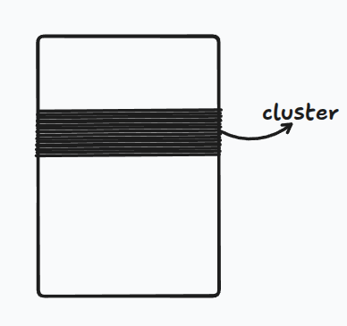
filled consecutive slots forming a cluster

Once you get a cluster of consecutive filled slots, it becomes a magnet. Any key that hashes anywhere into the cluster gets appended to the end, making the cluster longer, which makes it an even bigger magnet.

Under reasonable probabilistic assumptions, linear probing produces clusters of size $\Theta(\log n)$ when $\alpha < 0.99$ . That means search and insert degrade to $O(\log n)$ , not constant.

Satisfies permutation. Fails at load balancing. Avoid if you care about performance.

Double Hashing

$h(k,\ i) = (h_1(k) + i \cdot h_2(k)) \bmod m$

Use two independent hash functions. The step size between probes is now $h_2(k)$ , different for every key. Clusters can't form the same way because different keys bounce around differently.

To guarantee the permutation property: $h_2(k)$ and $m$ must be relatively prime, no common factors.

The easiest way to ensure this:

$m = 2^r \quad \text{and} \quad h_2(k) \text{ is always odd}$

An even step size on an even-sized table would only visit half the slots. Odd step + power-of-2 table → guaranteed full permutation.

Much better load balancing. Good in practice. This is what you actually use.

How Fast Is It?

We need an assumption called the Uniform Hashing Assumption:

Each key is equally likely to have any of the $m!$ possible permutations of slots as its probe sequence.

This is basically impossible to achieve perfectly, but double hashing gets close.

Under this assumption, the expected number of probes for an insert is:

$\leq \frac{1}{1 - \alpha}$

where $\alpha = n/m$ is the load factor.

Intuition for where this comes from:

The probability that your first probe lands on an empty slot is:

$\frac{m - n}{m} = 1 - \alpha$

Assuming the worst, that every trial has this same probability of success — the expected number of trials is:

$\frac{1}{1 - \alpha}$

That's the same as a geometric distribution with success probability $1 - \alpha$ .

$\alpha$	Expected probes
$0.5$	$2$
$0.9$	$10$
$0.99$	$100$

As $\alpha \to 1$ the table chokes. In practice, keep $\alpha \leq 0.5$ . Once you cross that, resize, double the table and rehash everything.

Open Addressing vs Chaining

	Chaining	Open Addressing
Memory	Extra (pointers + nodes)	Just one array
Max load factor	Can exceed 1	Must stay $< 1$
Practical sweet spot	$\alpha \approx 1$	$\alpha \leq 0.5$
Delete	Simple	Needs `DELETED` flag
Cache performance	Poor (pointer chasing)	Great (sequential memory)

Open addressing wins on memory and cache behavior. Chaining is more forgiving when the table gets crowded.

Cost Summary

Operation	Expected Time
Insert	$O\!\left(\frac{1}{1-\alpha}\right)$
Search	$O\!\left(\frac{1}{1-\alpha}\right)$
Delete	$O\!\left(\frac{1}{1-\alpha}\right)$

Keep $\alpha$ constant (by resizing) → all operations stay O(1).

REF

Based on MIT 6.006 lecture on Open Addressing.