Binary Trees

Personal notes on one of the most elegant ideas in computer science.🌳

Think about the data structures we usually reach for — arrays, linked lists, dynamic arrays, sorted arrays, hash tables(dictionary). Each one is brilliant at something and hopeless at something else, and there are two problems in particular where none of them really shine. The first is maintaining items in a chosen order while still being able to insert, delete, and access at arbitrary positions: linked lists can't even reach the middle without walking there step by step, and arrays can jump to the middle instantly but punish every insertion with a costly shift of everything after it. The second is maintaining items keyed for lookup, where hash tables crush exact searches but go blank the moment you ask "what's the next key after this one?", while sorted arrays answer those nearest-neighbor questions beautifully via binary search but collapse under dynamic updates.

Get all of it — order-based access, nearest-neighbor queries, dynamic inserts and deletes — in O(log n) time.

Binary trees are how we get there. In these notes I'll build up to O(h) time (where h is the tree's height). Making h itself logarithmic is a separate problem for another post.

Anatomy of a Binary Tree

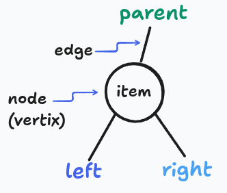
Each node carries four things:

• item — the actual payload
• parent — pointer upward
• left — pointer to the left child
• right — pointer to the right child

One node has no parent — that's the root.

An invariant worth internalizinxg:

node.left.parent  == node
node.right.parent == node

Parent pointers always mirror child pointers. If you break this, everything falls apart.

Why two pointers matter

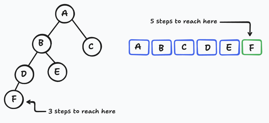
A singly-linked list node has one "next" pointer, so it can only form a straight line. The middle element is doomed to sit at linear depth from the head. Give each node two forward pointers and suddenly you can branch and branching structures can be shallow. A tree of n nodes can have height as small as log₂ n, meaning you can reach any node in just a handful of hops. That shallowness is the whole source of the speedup.

A shallow tree is one whose height is small relative to the number of nodes it contains...meaning the path from the root down to any leaf is short.

---

Terminology Cheat Sheet

Term	Meaning
Subtree of x	x plus every node descended from it
Ancestors of x	x's parent, grandparent, and so on up to the root
Descendants of x	everything below x
Leaf	a node with no children
Depth of x	edges on the path from x up to the root
Height of x	edges on the longest path from x down to a leaf
Height of the tree (h)	height of the root

Depth measures from the top down. Height measures from the bottom up.

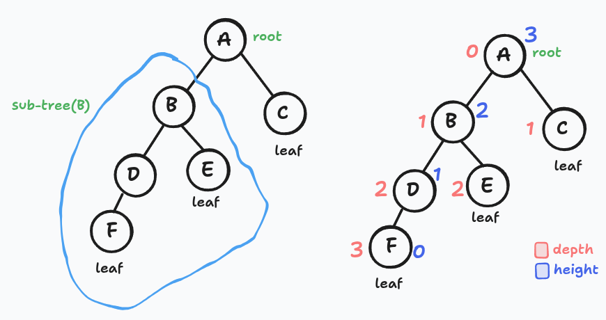
Height of C node? think? zero? yes, we count edges down (not vertices)

The Hidden Ordering: Traversal Order

Here's the crucial idea. Every binary tree implicitly defines a linear ordering of its nodes, defined recursively:

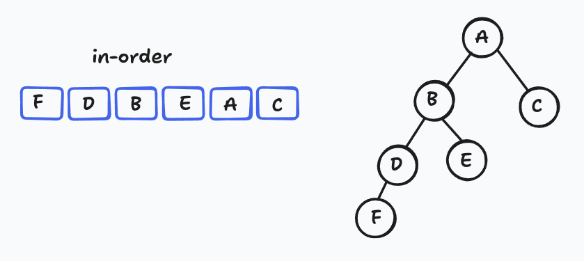
For every node x: everything in x's left subtree comes before x, and everything in x's right subtree comes after x.

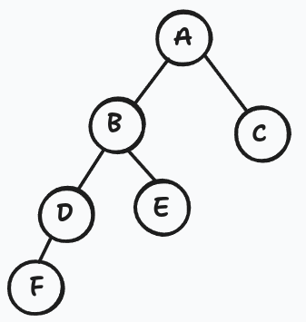
This is called the in-order traversal. For the tree in the sketch above, it reads: F, D, B, E, A, C.

The recursive algorithm is disarmingly short:

def traverse(x):
    if x is None: return
    traverse(x.left)
    visit(x)
    traverse(x.right)

⚠️ This ordering lives only in our heads. It is never stored explicitly. That's the whole trick — maintaining an explicit array of the order would be expensive, but a tree lets us manipulate the same ordering cheaply through pointer surgery.

---

The Operations

Every operation below runs in O(h) time. Keep the tree shallow and everything is fast.

Finding the first node of a subtree

To find the earliest node (in traversal order) among everything inside a subtree, walk left as far as possible:

def subtree_first(x):
    while x.left is not None:
        x = x.left
    return x

The leftmost descendant is always first. Symmetric logic gives you subtree_last — just walk right.

---

Successor: the next node in the whole tree

It is easy to know the successor from the in-order list. The successor of F is D and the successor of D is B.

Given some node, I want the very next one in traversal order across the entire tree. Two scenarios:

If the node has a right child, the successor is the first node of that right subtree:

return subtree_first(x.right)

If it doesn't, walk upward — but only through right-edges. Keep climbing as long as you're arriving at your parent from its right side. The first time you climb a left edge, that parent is your successor.

def successor(x):
    if x.right is not None:
        return subtree_first(x.right)
    while x.parent is not None and x is x.parent.right:
        x = x.parent
    return x.parent

The reasoning for the upward case: every time you climb a right edge, the parent is earlier than you (you were in its right subtree). The moment you climb a left edge, the parent is later than you — and nothing sits between you because you already ruled out having a right subtree.

predecessor is the mirror image.

---

Inserting a new node after an existing one

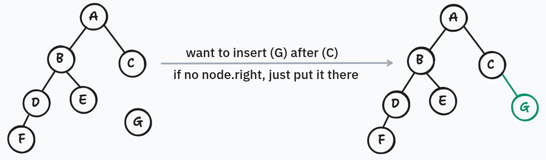
Given an existing node and a fresh node, place the fresh node immediately after the existing one in traversal order.

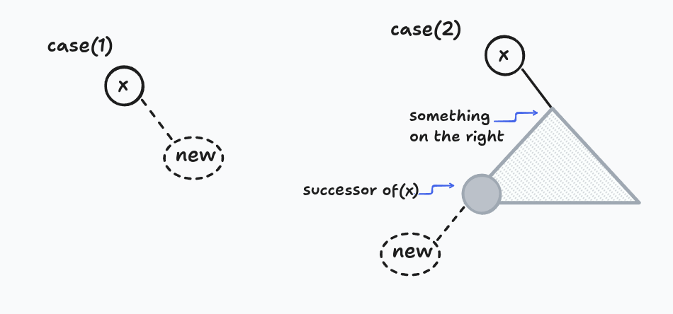
If the existing node has no right child, just attach the new node as its right child. Done.

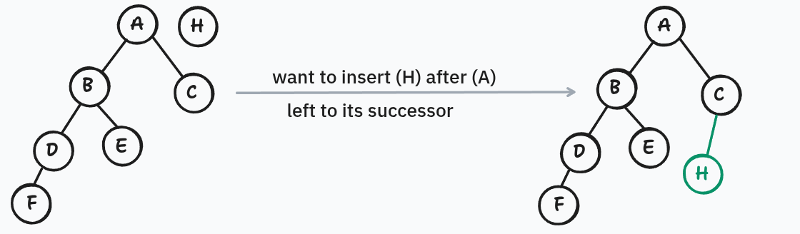
If it already has a right child, find its successor. That successor is guaranteed to have no left child (because subtree_first bottomed out going left). Attach the new node there as the successor's left child.

Either way, costs O(h). The "insert before" variant is perfectly symmetric.

---

Deleting a node

This one takes a little more care because you can't just erase a node in the middle of the tree — you'd orphan its children.

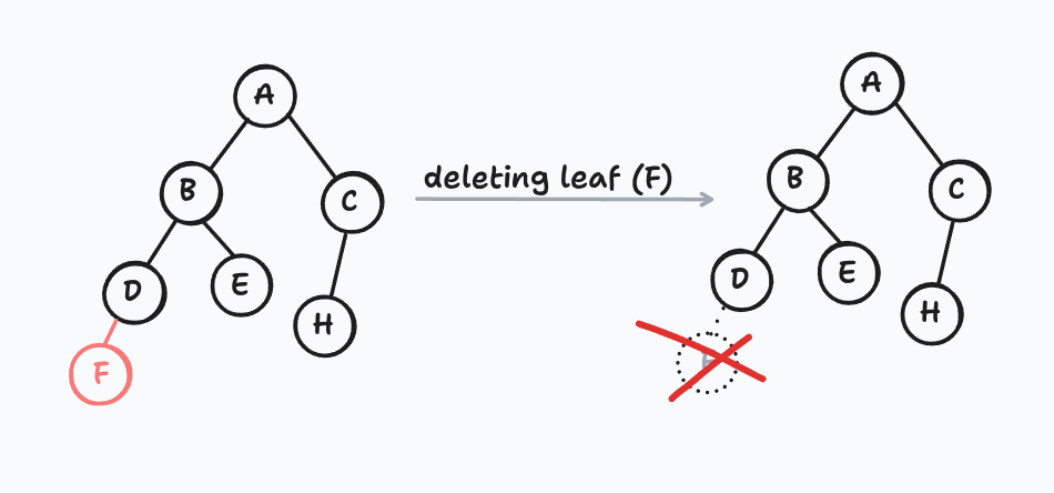
If it's a leaf, detach it. That's the base case.

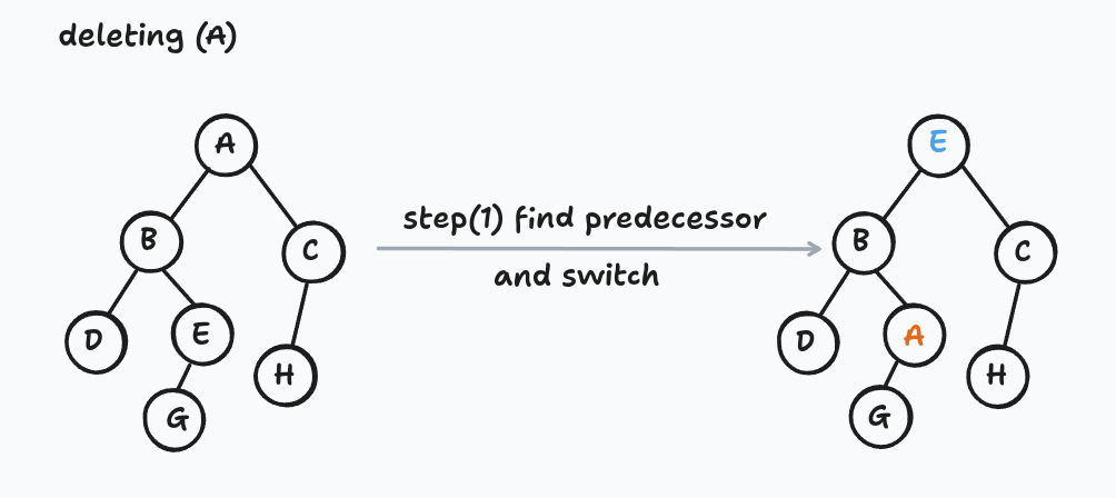
If it has a left child, swap its item with its predecessor's item, then recursively delete the predecessor. The predecessor sits somewhere down in the left subtree, so each recursive step pushes the problem further down.

If it has a right child but no left child, do the same thing with the successor.

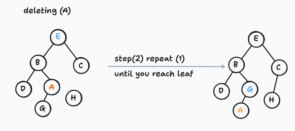
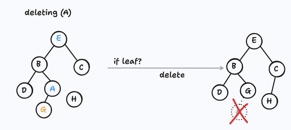
The node you originally wanted to delete ends up traveling down the tree (by item-swapping) until it reaches a leaf, at which point you snip it off.

Notice what's happening: the circles in the picture never move — we're rearranging the items stored inside them. This is the first operation where that distinction matters, and it's a technique worth remembering.

---

Turning Trees into Real Data Structures

Sequences

Interpret the traversal order as your sequence order. Position i corresponds to the i-th node visited. Getting random access in O(h) needs a little more machinery (subtree sizes), which is an another story for.

Sets — Binary Search Trees

Make the traversal order match the sorted order by key. This gives the celebrated BST property:

For every node, all keys in its left subtree are smaller than its own key, and all keys in its right subtree are larger.

Searching

Exactly binary search, expressed as a tree walk:

def find(x, key):
    while x is not None:
        if key < x.key:   x = x.left
        elif key > x.key: x = x.right
        else:             return x
    return None

Nearest-neighbor queries for free

When find walks off the bottom of the tree without a match, the last node it visited is already either the predecessor or the successor of the missing key — depending on whether the last step was "go right" or "go left." Getting the other neighbor is just one call to successor or predecessor.

This is the query hash tables can't answer, and we get it practically for free.

---

Cost Summary

Operation	Time
subtree_first / subtree_last	O(h)
successor / predecessor	O(h)
Insert after / before a node	O(h)
Delete a node	O(h)
find, find_prev, find_next	O(h)
Iterate every node	O(n)

Everything is shaped by h. The game now becomes: keep h small.

---

The Elephant in the Room (Another post for nerds)

Nothing I've said so far prevents you from building a catastrophically bad tree like this:

When h = n and every operation degenerates to linear time. So the real win — keeping h bounded by O(log n) no matter what — needs balancing. That's the topic I'll pick up in the next post: AVL trees, rotations, and how to make sure your tree never gets this lopsided.

Until then, the shape of the idea is already clear: two pointers per node, an implicit in-order traversal, and a handful of O(h) primitives that together handle almost every dynamic-ordering problem you can throw at them. Pretty elegant for something you can fit on a napkin.

REF

based on the lec and MIT open course